End-to-End Time Series Forecasting with AWS SageMaker
Note: The section Putting It All Together links to the GitHub repository containing the complete project source files. You can always return to this guide for a more detailed view of the project components.
Overview
In this post, we will train a times series model to forecast the weekly US finished motor gasoline products supplied (in thousands of barrels per day) from February 1991 to May 2005. This data set is available from the EIA website. The technology stack used in this project includes:
AWS ECR: a cloud-based container registry that makes it easy for us to store and deploy docker images. In this project, we use ECR to store the custom docker images for preprocessing, model training and inference.
AWS SageMaker: a fully managed service that allows data scientist to build, train, and deploy machine learning (ML) models with AWS cloud. In this project, we use SageMaker as a development environment to train a time series model and deploy the trained model artifacts as an inference endpoint.
AWS Lambda: a server-less compute service that runs our code in response to events and automatically manages the underlying compute resources for us. In this project, we use Lambda to invoke our deployed SageMaker inference endpoint.
AWS API Gateway: a fully managed service that makes it easy for us to create, publish, maintain, monitor, and secure APIs. In this project, we use API Gateway to create a REST API that will serve as a proxy between the client and the Lambda function, which in turn invokes the SageMaker inference endpoint.
In addition, we use the following tools to facilitate the development and deployment of our project:
Poetry: a tool used for managing dependencies and packaging the source code of the project.
Docker: a tool used for containerizing our applications code. In this project, we use docker to build custom images for model training and inference.
Hydra: an open-source framework for elegantly configuring complex applications. In this project, we use Hydra to manage the configurations— training meta-data, model configurations, compute resource specification, etc. — of our project.
Understanding IAM Roles and Users
Before we dive into the project, it is helpful to first review the concepts of IAM role and user. IAM stands for Identity and Access Management, which is an AWS service that helps us securely control access to AWS resources. In AWS, we often deal with two main types of IAM entities: roles and users. The following table summarizes the key differences between the two:
| Feature | IAM User | IAM Role |
|---|---|---|
| Definition | An entity that represents a human being working with AWS, typically for long-term access. | An identity with permissions that can be assumed by other entities (users, applications, AWS services). |
| Primary Use | For regular, direct interaction with AWS services. | For granting specific, temporary permissions for tasks or to AWS services. |
| Use Case in this Project | Represents individual team members (i.e., ourselves) working on the forecasting project, allowing them to access and manage AWS resources directly. | SageMaker Execution Role: Grants SageMaker permissions to access S3, manage EC2 instances, interact with ECR, etc. Lambda Execution Role: Allows Lambda to invoke SageMaker endpoint that hosts the trained models. |
| Policy Management | Permissions are generally managed through AWS managed policies or custom in-line policies directly attached to the user. | Roles are associated with AWS managed policies or custom in-line policies that define the permissions for the services assuming the role. |
Think of IAM users as our personal access points to AWS - they’re like our ID badges. On the other hand, IAM roles are more like keys that anyone (or any AWS service) can use to perform specific tasks, but only as needed.
Setting Up AWS Resources
To get started with the end-to-end project, we need to create the following resources in our AWS account:
- An ECR private repository to store the docker images for model training and inference. More details on how to create an ECR repository can be found in the official documentation. In this project, we create a private repository named
ml-sagemaker.

- An S3 bucket to store the training and test data as well as the trained model artifacts. See the official documentation on creating S3 buckets. For this project, we create a bucket named
yang-ml-sagemakerand a project keyforecast-project.

We can create all the above resources as the IAM user with the AdministratorAccess managed policy attached (i.e., not the default root user). Follow the official documentation to create such an administrative user. The administrative user has full access to all AWS services and resources in the account.
Although we can use a root or admin user for the remaining sections of this post, it is better practice, especially in team environments, to operate with a least-privilege user tailored to the project’s needs.
IAM User with Minimal Set of Permissions
In order to perform the actions— training, hosting, and deployment— required in this project, we need to create an IAM user and attach a policy with the following permissions: AmazonSageMakerFullAccess.
This is an AWS managed policy that provides full access to SageMaker via the AWS Management Console and SDK. It provides selected access to related services (e.g., S3, ECR, AWS CloudWatch Logs). The IAM user can be created from the IAM console of the administrative user. In the screen shot below:
The name of the IAM user is
forecast-project-userThe name of the AWS managed policy is
SageMakerFullAccess

We should also enable console access for this IAM user, so that we can login and manage our project resources from the AWS console. This can be done from the IAM console of the administrative user under the “Security credentials” tab.

Lambda Execution Role
A Lambda function’s execution role is an IAM role that allows a Lambda function to interact with other AWS services and resources. This role can be created via the IAM console by the administrative user. For this project, we need Lambda to integrate with two other AWS services:
SageMaker: to invoke the endpoint hosting the trained model
CloudWatch: to log the Lambda function’s execution for monitoring and troubleshooting
We make a resource restriction using the prefix forecast-, ensuring that the Lambda function can only invoke the endpoint hosting the trained model for this project. To set up this execution role, we follow a two-step process:
- Create an in-line policy called
forecast-lambda-policy(link) with the following permission, substituting forYOUR-AWS-ACOUNT-NUMBERor replacing it with the wildcard*:
{
    "Version": "2012-10-17",
    "Statement": [
        {
            "Sid": "InvokeSageMakerEnpoint",
            "Effect": "Allow",
            "Action": [
                "sagemaker:InvokeEndpoint"
            ],
            "Resource": "arn:aws:sagemaker:*:YOUR-AWS-ACOUNT-NUMBER:endpoint/forecast-*"
        },
        {
            "Sid": "CloudWatch",
            "Effect": "Allow",
            "Action": [
                "logs:CreateLogGroup",
                "logs:CreateLogStream",
                "logs:PutLogEvents"
            ],
            "Resource": "*"
        }
    ]
}
- Create the execution role called
forecast-lambda-execution-rolewith the above policy attached:


SageMaker Execution Role
Before moving on to creating the SageMaker notebook instance, we also need to create an IAM role for SageMaker to use. This role is used to give SageMaker training jobs, notebook instances, and models access to other AWS services, such as S3, CloudWatch, and ECR.
This execution role is also important as we will be creating our lambda function and REST API within the SageMaker notebook instance; therefore, we need additional permissions beyond the scope of AmazonSageMakerFullAccess. Similar to the execution role for Lambda, this IAM role can also be created from the IAM console of the administrative user.
- Create an in-line policy called
forecast-sagemaker-policy(link) with the following permissions, substituting forYOUR-AWS-ACOUNT-NUMBERor replacing it with the wildcard*:
{
    "Version": "2012-10-17",
    "Statement": [
        {
            "Sid": "ECRPermissions",
            "Effect": "Allow",
            "Action": [
                "ecr:BatchGetImage",
                "ecr:BatchDeleteImage",
                "ecr:ListImages"
            ],
            "Resource": "arn:aws:ecr:*:YOUR-AWS-ACOUNT-NUMBER:repository/YOUR-ECR-REPOSITORY"
        },
        {
            "Sid": "ReadOnlyPermissions",
            "Effect": "Allow",
            "Action": [
                "lambda:GetAccountSettings",
                "lambda:GetEventSourceMapping",
                "lambda:GetFunction",
                "lambda:GetFunctionConfiguration",
                "lambda:GetFunctionCodeSigningConfig",
                "lambda:GetFunctionConcurrency",
                "lambda:ListEventSourceMappings",
                "lambda:ListFunctions",
                "lambda:ListTags",
                "iam:ListRoles"
            ],
            "Resource": "*"
        },
        {
            "Sid": "DevelopFunctions",
            "Effect": "Allow",
            "NotAction": [
                "lambda:PutFunctionConcurrency"
            ],
            "Resource": "arn:aws:lambda:*:YOUR-AWS-ACOUNT-NUMBER:function:forecast-*"
        },
        {
            "Sid": "PassExecutionRole",
            "Effect": "Allow",
            "Action": [
                "iam:ListRolePolicies",
                "iam:ListAttachedRolePolicies",
                "iam:GetRole",
                "iam:GetRolePolicy",
                "iam:PassRole",
                "iam:SimulatePrincipalPolicy"
            ],
            "Resource": "arn:aws:iam::YOUR-AWS-ACOUNT-NUMBER:role/forecast-lambda-execution-role"
        },
        {
            "Sid": "ViewLogs",
            "Effect": "Allow",
            "Action": [
                "logs:*"
            ],
            "Resource": "arn:aws:logs:*:YOUR-AWS-ACOUNT-NUMBER:log-group:/aws/lambda/forecast-*"
        },
        {
            "Sid": "ConfigureFunctions",
            "Effect": "Allow",
            "Action": [
                "lambda:CreateFunction",
                "lambda:DeleteFunction",
                "lambda:UpdateFunctionCode",
                "lambda:UpdateFunctionConfiguration",
                "lambda:InvokeFunction"
            ],
            "Resource": "arn:aws:lambda:*:YOUR-AWS-ACOUNT-NUMBER:*:*"
        },
        {
            "Sid": "ManageAPIGateway",
            "Effect": "Allow",
            "Action": [
                "apigateway:POST",
                "apigateway:GET",
                "apigateway:PUT",
                "apigateway:DELETE"
            ],
            "Resource": [
                "arn:aws:apigateway:*::/restapis",
                "arn:aws:apigateway:*::/restapis/*",
                "arn:aws:apigateway:*::/apikeys",
                "arn:aws:apigateway:*::/apikeys/*",
                "arn:aws:apigateway:*::/usageplans",
                "arn:aws:apigateway:*::/usageplans/*",
                "arn:aws:apigateway:*::/usageplans/*/*"
            ]
        },
        {
            "Sid": "InvokeAPIGateway",
            "Effect": "Allow",
            "Action": [
                "execute-api:Invoke"
            ],
            "Resource": "arn:aws:execute-api:*:YOUR-AWS-ACOUNT-NUMBER:*/*/POST/*"
        }
    ]
}
Here is a breakdown of the permissions in the above policy:
ECRPermissions: Allows managing images in an ECR repository named
ml-sagemaker, including getting, deleting, and listing images. This should be modified to theECRrepository created in the previous section.ReadOnlyPermissions: Grants read-only access to various Lambda-related actions, including viewing function details and listing functions and roles.
DevelopFunctions: Provides broader permissions for Lambda functions prefixed with
forecast-, except for changing function concurrency settings. (Notice the use ofNotAction).PassExecutionRole: Enables passing a specific IAM role (
forecast-lambda-execution-role) to AWS services for executing functions.ViewLogs: Grants full access to logs associated with Lambda functions starting with
forecast-.ConfigureFunctions: Provides permissions to create, delete, update, and invoke Lambda functions across all regions for the specified AWS account.
ManageAPIGateway: Allows managing REST APIs in API Gateway, including CRUD operations on APIs.
InvokeAPIGateway: Grants permission to invoke POST methods on API Gateway endpoints.
- Create the execution role called
forecast-sagemaker-execution-rolewith two policies attached:
The first policy is the AWS managed policy
AmazonSageMakerFullAccessThe second policy is the in-line policy created above


We will need to reference this execution role when creating the SageMaker notebook instance below.
Optional: Lifecycle Configuration Script & Secret for Github
Optionally, we can enhance our SageMaker notebook instance with a lifecycle configuration script. This script runs both at the creation of the notebook instance and each time it starts, allowing us to install extra libraries and packages beyond the default setup. We can even configure an IDE like VSCode in the notebook instance. For guidance on setting up VSCode, check out my previous post.
Additionally, linking our SageMaker notebook to a Git repository (either public or private) is possible and beneficial for version control and collaboration. For private repositories, we’ll need to create a personal access token and store it in AWS Secrets Manager. This token is then used to establish a secure connection to the repository. Detailed steps can be found in the SageMaker documentation.
SageMaker Notebook Instance
For connecting with a Github repo, if we did not create a PAT and store it with Secret Manager in the previous step, we would either have to log back in and create the secret with the administrative user or grant permissions to do so to the forecast-project-user IAM user. If we did create a PAT and stored it with Secret Manager, we can first create a github repo for the project:

Once the github repo is created, we create a SageMaker notebook instance from the SageMaker console of the forecast-project-user IAM user. The notebook instance is used as our primary development environment for model training and inference.


As for the instance type, we can choose ml.t3.medium, which comes with 2 vCPU’s and 4 GiB of memory at \(\$0.05\) per hour on-demand. The instance type can be changed later if needed, but it is recommend to start small with any development instances and utilize and processing and training jobs with more compute for actual workloads. For more details on pricing, refer to the SageMaker pricing page.
For this project, we will connect to Github from within the notebook instance; this is because we will be creating a project directory from scratch.
Setting Up Project in the SageMaker Notebook Instance
Every SageMaker notebook instance comes equipped with a dedicated storage volume. To set up our project, we will begin by creating a shell script within this storage. From this point on, you could either use JupyerLab (provided by SageMaker) or VSCode, which we optionally installed via the lifecycle configuration above.

Open the terminal, navigate to the SageMaker directory, and create a shell script:
$ cd /home/ec2-user/SageMaker
# You can use any text editor of your choice
$ nano create_project.sh
Copy and paste the following commands into the script:
#!/bin/bash

# Activate conda environment
source ~/anaconda3/etc/profile.d/conda.sh && conda activate python3 && pip3 install poetry

# This creates a new project with directories src and tests and a pyproject.toml file
poetry new forecast-project --name src
# Use sed to update the Python version constraint in pyproject.toml
sed --in-place 's/python = "^3.10"/python = ">=3.10, <3.12"/' pyproject.toml

# Install project, test, notebook dependencies
cd forecast-project
poetry add "pandas[performance]==1.5.3" "hydra-core==1.3.2" "boto3==1.26.131" \
           "pmdarima==2.0.4" "sktime==2.24.0" "statsmodels==0.14.0" "statsforecast==1.4.0" \
           "xlrd==2.0.1" "fastapi==0.104.1" "joblib==1.3.2" "uvicorn==0.24.0.post1"
poetry add "pytest==7.4.2" --group test
poetry add "ipykernel==6.25.2" "ipython==8.15.0" "kaleido==0.2.1" "matplotlib==3.8.0" --group notebook

poetry install
The script above accomplishes the following:
Activates the pre-installed
python3conda environment and installs PoetryCreates a poetry-managed project named
forecast-projectInstalls dependencies into separate groups:
- Packages used for training
- Packages used for testing
- Packages used in the jupyter notebook for interactive development
We employ exact versioning (==) for all dependencies. This approach isn’t about futureproofing the package. Instead, the objective of packaging the training code is to firmly lock in the set of dependencies that have proven to work, ensuring consistency during testing, training, and notebook usage.
Installs the
srcpackageModifies the Python version constraint in
pyproject.toml(as of the time of writing the article, the python 3 version of thepython3conda environment is3.10.12)
Run the script:
$ bash create_project.shTo confirm that the src package has been installed in the Conda environment
$ source activate python3
$ conda list src
# Name Version Build Channel
src 0.1.0 pypi_0 pypiThe pyproject.toml file should resemble:
[tool.poetry]
name = "src"
version = "0.1.0"
description = ""
authors = ["Yang Wu"]
readme = "README.md"

[tool.poetry.dependencies]
python = ">=3.10, <3.12"
pandas = {version = "1.5.3", extras = ["performance"]}
hydra-core = "1.3.2"
boto3 = "1.26.131"
pmdarima = "2.0.4"
sktime = "0.24.0"
statsmodels = "0.14.0"
xlrd = "2.0.1"
statsforecast = "1.4.0"
fastapi = "0.104.1"
joblib = "1.3.2"
uvicorn = "0.24.0.post1"

[tool.poetry.group.test.dependencies]
pytest = "7.4.2"

[tool.poetry.group.notebook.dependencies]
ipykernel = "6.25.2"
ipython = "8.15.0"
kaleido = "0.2.1"
matplotlib = "3.8.0"

[build-system]
requires = ["poetry-core"]
build-backend = "poetry.core.masonry.api"
To enable version control the project, you may refer to the following section of my previous post on using transformers for tabular data.
Hydra Configuration
Thus far, we’ve established several AWS resources, including an S3 bucket and a SageMaker notebook. As our project becomes more intricate, it can be challenging to keep track of all these resources, especially elements like names (such as user name, project S3 key, S3 bucket name, etc.) and paths (like the project directory and its subdirectories). This issue becomes even more critical as we start developing our training and inference logic, which come with their own configuration requirements.
To tackle this challenge, we’ll employ Hydra for managing our project’s configurations. Instead of hardcoding configurations directly into scripts or notebooks, which can be prone to errors when changes occur frequently during development, Hydra allows us to store configurations in a structured and organized manner.
Create a config directory and a main.yaml file in the src directory:
$ cd forecast-project
$ mkdir src/config && touch src/config/main.yaml
The main.yaml file functions as the central hub for all configurations, serving as the primary reference point for a wide range of project settings. These settings encompass paths, AWS resources and names, meta data, raw data url, and more. Edit the main.yaml file and add the following:
# AWS config
s3_bucket: YOUR-S3-BUCKET
s3_key: YOUR-PROJECT-KEY
ecr_repository: YOUR-ECR-REPOSITORY
model_dir: /opt/ml/model
output_path: s3://YOUR-S3-BUCKET/YOUR-PROJECT-KEY/models
code_location: s3://YOUR-S3-BUCKET/YOUR-PROJECT-KEY/code
volume_size: 30
# File system
project_dir_path: /home/ec2-user/SageMaker/YOUR-PROJECT-KEY
src_dir_path: /home/ec2-user/SageMaker/YOUR-PROJECT-KEY/src
notebook_dir_path: /home/ec2-user/SageMaker/YOUR-PROJECT-KEY/notebooks
docker_dir_path: /home/ec2-user/SageMaker/YOUR-PROJECT-KEY/docker
# Meta data for ingestion and uploading to s3
raw_data_url: https://www.eia.gov/dnav/pet/hist_xls/WGFUPUS2w.xls

# Meta data
freq: W-FRI
m: 52.18
forecast_horizon: 26 # Forecast horizon 26 weeks or ~ 6 months
max_k: 10 # Maximum number of fourier terms to consider
cv_window_size: 417 # Selected to ensure 100 train-val splits
test_window_size: 512 # Selected to test only 5 train-val splits
step_length: 1 # Step size for rolling window
conf: 0.95 # Confidence level for prediction intervals

# Processing job configuration
preprocess_base_job_name: processing-job
preprocess_input: /opt/ml/processing/input
preprocess_output: /opt/ml/processing/output
preprocess_instance_count: 1
preprocess_instance_type: ml.t3.medium
preprocess_entry_point: preprocess_entry.py
preprocess_counterfactual_start_date: '2013-01-01'

# Training job configuration
train_base_job_name: training-job
train_instance_count: 1
train_instance_type: ml.m5.xlarge
train_entry_point: train_entry.py

# Hyperparameter optimization
base_tuning_job_name: tuning-job
max_jobs: 20
max_parallel_jobs: 10
objective_type: Minimize
objective_metric_name: 'MSE'
strategy: Bayesian

# Spot training
use_spot_instances: true
max_run: 86400
max_wait: 86400 # This should be set to be equal to or greater than max_run
max_retry_attempts: 2
checkpoint_s3_uri: s3://YOUR-S3-BUCKET/YOUR-PROJECT-KEY/checkpoints

# Serving configuration
serve_model_name: forecast-model
serve_memory_size_in_mb: 1024  # 1GB increments: 1024 MB, 2048 MB, 3072 MB, 4096 MB, 5120 MB, or 6144 MB
serve_max_concurrency: 5 # Maximum number of concurrent invocation the serverless endpoint can process
serve_initial_instance_count: 1
serve_instance_type: ml.t3.medium
serve_endpoint_name: forecast-endpoint
serve_volume_size: 10

# Lambda
lambda_source_file: lambda_function.py
lambda_function_name: forecast-lambda
lambda_handler_name: lambda_function.lambda_handler
lambda_execution_role_name: forecast-lambda-execution-role
lambda_python_runtime: python3.10
lambda_function_description: Lambda function for forecasting gas product
lambda_time_out: 30
lambda_publish: true
lambda_env_vars:
  - SAGEMAKER_SERVERLESS_ENDPOINT: forecast-endpoint

# API Gateway
api_gateway_api_name: forecast-api
api_gateway_api_base_path: forecast
api_gateway_api_stage: dev
api_gateway_api_key_required: true
api_gateway_api_key_name: forecast-api-key
api_gateway_enabled: true # Caller can use this API key
api_gateway_usage_plan_name: forecast-api-usage-plan

defaults:
  - _self_
This yaml file can be adapted to fit the needs of different projects. Make sure that the placeholders— YOUR-S3-BUCKET, YOUR-PROJECT-KEY, and YOUR-ECR-REPOSITORY are replaced with appropriate values.
Checkpoint I
At this juncture, the project directory should resemble:
.
├── poetry.lock
├── pyproject.toml
├── README.md
├── src
│   ├── config
│   │   └── main.yaml
│   └── __init__.py
└── tests
    └── __init__.py
Exploratory Data Analysis
Create a notebooks directory in the root directory of the project, then create a notebook named eda.ipynb inside the notebooks directory:
$ mkdir notebooks && cd notebooks && touch eda.ipynbThe code blocks of the following sub-sections are all assumed to be executed inside the eda.ipynb notebook. Note: the kernel of the notebook should be set to the conda environment, python3, in which we installed our project dependencies.
Hydra
To set up Hydra for the notebook, all we need to do is initializing it with a configuration path relative to the caller’s current working directory. In this case, the caller is the eda.ipynb notebook, and the configuration path is ../src/config. We’ll also need to specify the version base and job name for the notebook. Lastly, we’ll convert the Hydra configuration to a dictionary for easy access:
core.global_hydra.GlobalHydra.instance().clear()
initialize(version_base='1.2', config_path='../src/config', job_name='eda')
config = OmegaConf.to_container(compose(config_name='main'), resolve=True)
Data
To download the raw data from the Energy Information Administration website to the current working directory (i.e. notebooks):
!wget -q {config['raw_data_url']} -O gas_data.xlsRead in the excel file:
gas_data = pd.read_excel(
    'gas_data.xls',
    sheet_name='Data 1',
    header=2, # The column names start on the 3rd row
    dtype={'Date': np.datetime64},
    index_col='Date'
)

gas_data.columns = ['gas_product']

gas_data.shape
(1707, 1)Check for missing values and duplicate values:
assert gas_data['gas_product'].isna().sum() == 0
assert gas_data.index.duplicated(keep=False).sum() == 0
In this project, we will try to forecast the next 6 months of gas products, which means that the last \(\sim6\) months (or \(\sim26\) weeks) of data will become the test set. All EDA steps will be conducted on the training set. The forecast horizon we choose here is arbitrary, and can be changed in the configuration file.
train, test = pm.model_selection.train_test_split(gas_data, test_size=config['forecast_horizon'])
print(f'The training period is {train.index.min().strftime("%Y-%m-%d")} to {train.index.max().strftime("%Y-%m-%d")}')
print(f'The test period is {test.index.min().strftime("%Y-%m-%d")} to {test.index.max().strftime("%Y-%m-%d")}')
The training period is 1991-02-08 to 2023-04-21
The test period is 2023-04-28 to 2023-10-20Fundamental Questions in Time Series Analysis
To gain a comprehensive understanding of our time series data, we start by addressing two fundamental questions:
Is the time series stationary? From the book “Time Series Analysis with Applications in R” by Jonathan D. Cryer and Kung-Sik Chan (page 16):
To make statistical inferences about the structure of a stochastic process on the basis of an observed record of that process, we must usually make some simplifying (and presumably reasonable) assumptions about that structure. The most important such assumption is that of stationarity. The basic idea of stationarity is that the probability laws that govern the behavior of the process do not change over time. In a sense, the process is in statistical equilibrium. Specifically, a process \({Y_t}\) is said to be strictly stationary if the joint distribution of \(Y_{t_1}, Y_{t_2},..., Y_{t_n}\) is the same as the joint distribution of \(Y_{t_{1}– k}, Y_{t_{2}– k},..., Y_{t_a{n}– k}\) for all choices of time points \(t_1, t_2,..., t_n\) and all choices of time lag k.
In practice, we usually answer the question of stationarity using the weak definition. That is, a time series \(Y_{t}\) is weakly stationary if
- The mean function is constant over time
- \(\gamma_{t, t-k}=\gamma_{0, k} \quad\) for all time \(t\) and lag \(k\)
Is the time series a white noise (i.e., a sequence of independent, identically distributed random variables)? The white noise is an example of a stationary process; most importantly, if the data is confirmed to be white noise, we cannot reasonably forecast such time series.
Time Plot, ACF, & PACF
To answer the above questions, we rely on three essential plots:
Time Plot: this is simply the time series (y-axis) over time (x-axis). Things to look for in this plot are:
What is the baseline (grand mean) of the series over the sampling period?
Is there a trend (i.e. positive or negative slope) over time?
Is there a noticeable (and consistent) seasonal pattern in the time series? There is a subtle difference between seasonal and any cyclical patterns; the latter do not have to be consistent. In other words, seasonal patterns (temperature fluctuation over the course of a single year) are predictable and cyclical (economic expansion, contraction, and trough) are not consistent in the long run. This is why it is important to examine the time plot of the series over time.
If there are repeated seasonal patterns, do the variances change over time? In other words, over time, do the vertical distances of the seasonal fluactuaions become larger or smaller?
ACF plot or correlogram: the (sample) autocorrelation function, \(r_{k}\), at lag \(k\), for the observed time series \(Y_1, Y_2, \ldots, Y_n\) is given as follows:
\[\begin{equation*} r_k=\frac{\sum_{t=k+1}^n\left(Y_t-\bar{Y}\right)\left(Y_{t-k}-\bar{Y}\right)}{\sum_{t=1}^n\left(Y_t-\bar{Y}\right)^2} \quad \text{for } k=1,2, \ldots \end{equation*}\]
where:
- \(Y_1, Y_2,..., Y_n\) is times series
- \(\bar{Y}\) is the grand mean of the entire series
- \(\sum_{t=1}^n\left(Y_t-\bar{Y}\right)^2\) is the grand sum of squares (i.e., there are \(n\) squared terms)
- \(\sum_{t=k+1}^n\left(Y_t-\bar{Y}\right)\left(Y_{t-k}-\bar{Y}\right)\) is the sum of \(n - k\) cross products
In this plot, we are looking for significant correlation coefficients between the time series and different of lagged values of itself to determine if there are seasonal patterns or if the series is white noise.
If seasonal patterns are present, the plot of the sample ACF often exhibits sinusoidal patterns.
If the time series is white noise, the correlogram displays statistically insignificant autocorrelation coefficients \(r_{k}\) for most (if not all) lag \(k\).
The ACF plot can often used to graphically determine the orders of the (non-seasonal) \(MA(q)\) and (seasonal) \(MA(Q)\) components of the (S)ARIMA model. It can be shown that, for \(MA(q)\) and \(MA(Q)\) processes, the autocorrelation function is theoretically zero for non-seasonal lags beyond \(q\) or seasonal lags beyond \(Q\). As a result, the sample ACF plot can be a good indicator for the \(q\) or \(Q\) at which the significant lags cut off.
PACF plot: the (sample) partial autocorrelation, denoted as \(\phi_{k k}\), is defined as
\[\begin{equation*} \phi_{k k}=\frac{\rho_k-\sum_{j=1}^{k-1} \phi_{k-1, j} \rho_{k-j}}{1-\sum_{j=1}^{k-1} \phi_{k-1, j} \rho_j} \end{equation*}\]
where
\(\phi_{k k}\) represents the correlation between \(Y_t\) and \(Y_{t − k}\) after removing the effect of the intermediate lag values (\(Y_{t − 1}, Y_{t − 2}, Y_{t − 3},..., Y_{t − k + 1}\))
\(\phi_{k, j}=\phi_{k-1, j}-\phi_{k k} \phi_{k-1, k-j} \quad \text { for } j=1,2, \ldots, k-1\)
The PACF has the same property for \(AR\) processes as that of the ACF for \(MA\) processes. Theoretically, the partial correlation coefficient at lag \(k\) becomes zero beyond the the appropriate orders \(p\) and \(P\). Thus, the PACF plot is often used to identify the orders of the (non-seasonal) \(AR(p)\) and (seasonal) \(AR(P)\) components of the (S)ARIMA model.
General Behavior of the ACF and PACF for ARMA Models
| AR \(p\) | MA \(q\) | ARMA \(p, q\), \(p>0\), and \(q>0\) | |
|---|---|---|---|
| ACF | Tails off | Cuts off after lag \(q\) | Tails off |
| PACF | Cuts off after lag \(p\) | Tails off | Tails off |
Source: Time Series Analysis With Applications in R (page 116)
Although the table above describes the general behaviors for (non-seasonal) ARMA models, the same principles apply when determining the orders of the seasonal components \(P\) and \(Q\) for a (S)ARMA model. However, instead of looking for characteristics like tailing off or cutting off beyond \(p\) and \(q\) lags, we focus on these characteristics over seasonal lags. For weekly data, where the seasonality period is approximately \(365.25/7 \approx 52.18\), we can pay attention to lag 52, 104, and so on.
In terms of the number of lags to plot, we use a rule-of-thumb based on the following post by Rob Hyndman.
lags = np.min([2 * (365.25 / 7), (gas_data.shape[0] / 5)])

fig, ax = plot_correlations(
    series=gas_data,
    lags=lags,
    zero_lag=False,
    suptitle='Weekly U.S. Product Supplied of Finished Motor Gasoline'
)
fig.set_size_inches((16, 5))
plt.show()
ACF
fig = plot_acf(
    x=gas_data,
    lags=lags,
    zero=False
)
fig.set_size_inches(12, 6)
plt.axvline(x=52, color='r', linestyle='--', label='Lag 52')
plt.axvline(x=104, color='g', linestyle='--', label='Lag 104')
plt.legend()
plt.show();
PACF
fig = plot_pacf(
    x=gas_data,
    lags=lags,
    zero=False
)
fig.set_size_inches(12, 6)
plt.axvline(x=52, color='r', linestyle='--', label='Lag 52')
plt.axvline(x=104, color='g', linestyle='--', label='Lag 104')
plt.legend()
plt.show();
Observations
The following observations can be made:
The time series is definitely non-stationary with both weekly seasonality and non-constant trends, as indicated by the sinusoidal patterns in the ACF (i.e., the peak-to-peak patterns last about \(\sim52\) lags).
The trends can be more clearly observed by plotting the yearly averages:
gas_data.resample('YS').mean().plot(y='gas_product', figsize=(7, 5), title='Average Gas Product by Year');
- The yearly variances of the series, with the exception of year 2020 (i.e., COVID-19), appear relatively stable, but we can further stabilize the variances with a data transformation.
gas_data.resample('YS').var().plot(y='gas_product', figsize=(7, 5), title='Variance of Gas Product by Year');
The confirmed seasonal period is quite long, i.e., \(m\approx52.18\). Instead of the (S)ARIMA model, which is designed for shorter seasonal periods such as 12 for monthly data and 4 for quarterly data, we can train a harmonic regression model. With this approach,
\[\begin{equation*} y_t=a+\sum_{k=1}^K\left[\alpha_k \sin (\frac{2 \pi k t}{m})+\beta_k \cos (\frac{2 \pi k t}{m})\right]+N_t \end{equation*}\]
seasonal patterns are modeled using Fourier terms
short-term patterns are modeled by the \(N_{t}\) ARMA process
the smoothness of the seasonal pattern can be controlled by the frequency hyperparameter \(K\), which is the number of Fourier sin and cos pairs; the seasonal pattern is smoother for smaller values of \(K\), which can be tuned using time-series cross-validation
Finally, the devastating effect of the COVID-19 pandemic on the gasoline industry is fairly noticeable in the time plot for year 2020. These extreme values should be addressed before training any model. There may be many possible ways to handle these outliers, but we will revert to an approach of judgemental forecasting.
gas_data.loc['2018':'2023'].plot(figsize=(15, 5), title='Gas Product (2019 - 2023)');
Handling COVID-19 with Scenario-Based Forecasting
It can be argued that the sudden drop of gasoline products observed in the data (and in the time plot) represents a structural break that is caused by the COVID-19 pandemic. According to the research conducted by Athanasopoulos et al. (2023) and published in the Journal of Travel Research, Volume 62, Issue 1, the biggest challenge presented by the COVID-19 pandemic on any forecasting tasks is an increased level of uncertainly:
From a statistical modelling and forecasting perspective, these disruptions cause unique challenges. The pandemic has meant that we cannot extrapolate the strong and persistent signals observed in historical tourism time series. The structural break is deep and the path to recovery remains extremely uncertain.
The authors in this paper argue that historical data from the COVID-19 years cannot be used to forecast without first addressing this structural breakdown:
… the effect of the COVID-19 pandemic is such that historical data cannot be used to project forward without explicitly accounting for the depth and the length of the structural break caused by COVID-19, and the subsequent unknown and unprecedented path to recovery. Both the depth and length of the effect of the pandemic are extremely challenging or even impossible to estimate and predict statistically, and therefore we revert to a novel approach of judgemental forecasting.
In this project, we will develop our own judgmental forecasting methodology, which includes the following steps:
- Identify outliers using robust Season-Trend decomposition with LOESS weighting, where any outliers will be detected in the remainder series.
- Determine the outlier with the earliest and latest dates within the COVID-19 years (i.e., Jan 2020 onward). These effectively serve as proxies for the length of the structural break.
- Utilize STL forecasting, which employs the seasonal naive method for forecasting the decomposed trend, seasonal, and residual components separately; these forecasts are then combined to predict gasoline product for all observations between the dates identified in the previous step.
- Replace all values between the earliest and latest dates within the COVID-19 years with the forecast generated by the model.
This approach allows us to consider a counterfactual scenario had the COVID-19 pandemic never occurred. Any subsequent models trained on this “counterfactual” data generate forecasts that can be regarded as recovery trajectories. In other words, these forecasts represent the gasoline production levels that might have been attained if the pandemic had not happened, and they should serve as the benchmark that producers should aim to return to.
The objective is to provide more dependable scenario-based forecasts. Consequently, the step involving the training of a model to predict the COVID-19 data will be treated as a hyperparameter in itself, fine-tuned using time series cross-validation.
Decomposition
m = (365.25 / 7)
decomp_result = STL(endog=pd.Series(train['gas_product'], name='Seasonal-Trend Decomposition of Gas Product'), period=int(np.floor(m)), robust=True).fit()
fig = decomp_result.plot()
fig.set_size_inches(12, 8)
plt.show();
Outlier Detection
We define outliers as observations whose residuals are greater than three times the interquartile range (IQRs) of the middle 50% of the data.
resid_75 = np.quantile(decomp_result._resid, 0.75)
resid_25 = np.quantile(decomp_result._resid, 0.25)
resid_iqr = resid_75 - resid_25

# Indices of outliers
outlier_indices = np.logical_or((decomp_result._resid > resid_75 + 3 * resid_iqr), (decomp_result._resid < resid_25 - 3 * resid_iqr))
outlier_indices.sum()46Print the earliest and latest dates of the outliers within the COVID-19 years:
earliest = train.loc[(outlier_indices)].loc['2020'].index.min().strftime('%Y-%m-%d')
latest = train.loc[(outlier_indices)].index.max().strftime('%Y-%m-%d')
print(f'The outlier with the earliest date within the COVID-19 years is {earliest}')
print(f'The outlier with the latest date within the COVID-19 years is {latest}')
The outlier with the earliest date within the COVID-19 years is 2020-03-13
The outlier with the latest date within the COVID-19 years is 2022-08-19We will add a boolean column to the data set to flag outlying observations that should be substituted with forecasts:
train['covid_forecast'] = np.logical_and((train.index >= earliest), (train.index <= latest))
test['covid_forecast'] = False
Upload to S3
We can proceed by uploading the raw data, including the new boolean column, to S3. This step is crucial as it enables us to continue with the following tasks:
Train-test split
Forecasting COVID-19 data using historical data
We will perform these tasks using a SageMaker processing job.
# Save the outlier indices to the current directory
pd.concat([train, test], axis=0).to_csv('gas_data.csv', index=True)

# Upload both the raw data and the outlier indices to s3
sagemaker.s3.S3Uploader.upload('gas_data.csv', f's3://{config["s3_bucket"]}/{config["s3_key"]}/raw-data')

# Remove from the current directory
os.remove('gas_data.csv')
os.remove('gas_data.xls')
Checkpoint II
By the end of EDA, our project directory should look like this:
.
├── notebooks
│   └── eda.ipynb
├── poetry.lock
├── pyproject.toml
├── README.md
├── src
│   ├── config
│   │   └── main.yaml
│   └── __init__.py
└── tests
    └── __init__.py
Processing Job
To prepare the data for training, including generating a model-based counterfactual data set, we will use a SageMaker processing job. The diagram below provides a visual representation of how SageMaker orchestrates a processing job. SageMaker takes our processing script, retrieves our data from S3 (if applicable), and then deploys a processing container. This container image can be a built-in SageMaker image or a custom one we provide. The advantage of processing jobs is that Amazon SageMaker handles the underlying infrastructure, ensuring resources are provisioned only for the duration of the job and then reclaimed afterward. Upon completion, the output of the processing job is stored in the specified Amazon S3 bucket.

Two additional resources to learn about SageMaker processing jobs:
For other example usages, check out the official Amazon SageMaker Examples documentation page.
For documentation on API, see here.
Processing Entry Script
Create a preprocess_entry.py (link) script in the src directory. Here is a summary of the script:
| Section | Description |
|---|---|
| Script Overview | The script preprocess_entry.py contains the logic for forecasting COVID-19 data using STL forecasting with naive methods for different components. It operates within AWS SageMaker as a processing job and includes a preprocess pipeline with a log transformation followed by STL forecasting for COVID-19 data. |
| Key Libraries Used | - pandas: For data manipulation and analysis. - numpy: For numerical operations. - sktime: For advanced time series forecasting, particularly STL and naive forecasting methods. - argparse: For command-line option and parsing hyperparameters passed to the preprocessing script at run-time. - hydra: For managing configuration files. - logging: For generating log messages. - warnings: For handling warnings during script execution. |
| Main Functionalities | 1. Data Preparation: Loads and preprocesses gas product data, including the boolean indicator for outlaying COVID-19 observations. 2. Model Configuration and Forecasting: Sets up STL forecasting with naive methods for trend, seasonality, and residuals, which are forecast separately and combined to forecast these outlaying COVID-19 observations. 3. Data Splitting: Divides the data into training and testing sets based on a specified forecast horizon. 4. Data Saving: Saves processed data to disk, with an option to skip saving in test mode. |
| STL Forecasting with Naive Methods | Employs STL forecasting, decomposing the time series into trend, seasonal, and residual components, each forecasted using the naive method with strategy = mean. This approach is encapsulated in a forecast function that manages the forecasting process. |
| Configuration Management | Utilizes Hydra for managing configuration parameters, allowing for easy adjustment of settings separated from the code. Configuration parameters are accessed from a dictionary object. |
| Testing with Local Mode | Includes a --test_mode argument for local testing, which reduces data size and skips saving results to disk. This feature is useful for testing the script in a local environment before deploying it to AWS SageMaker. |
Custom Docker Image for Processing
To facilitate a streamlined data processing workflow, we will create a custom Docker image. In this project, we will not only build an image to process our data but also build two other images to train and serve our model. To manage the creation and deployment of these images, we will create a parameterized bash script. First, create a docker directory in the root directory of the project and a build_and_push.sh (link) script that takes three arguments:
image_tag: tag of the docker imagemode: one of ‘preprocess’, ‘train’, ‘serve’ecr_repo: name of the ECR private repository
The script below automates the task of building docker images for any of the specific task— preprocess, train, or serve— and pushes it to the ECR repository we created earlier.
#!/bin/bash

# Always anchor the execution to the directory it is in, so we can run this bash script from anywhere
SCRIPT_DIR=$(python3 -c "import os; print(os.path.dirname(os.path.realpath('$0')))")

# Set BUILD_CONTEXT as the parent directory of SCRIPT_DIR
BUILD_CONTEXT=$(dirname "$SCRIPT_DIR")

# Check if arguments are passed, otherwise prompt
if [ "$#" -eq 3 ]; then
    image_tag="$1"
    mode="$2"
    ecr_repo="$3"
else
    read -p "Enter the custom image tag name: " image_tag
    read -p "Select one of preprocess, train, or serve: " mode
    read -p "Enter the ECR repository name: " ecr_repo
fi

# Check if the image tag is provided where [-z string]: True if the string is null (an empty string)
if [ -z "$image_tag" ] || [ -z "$ecr_repo" ]; then
  echo "Please provide both the custom image tag name and the ECR repository name."
  exit 1
fi

# Choose Dockerfile based on mode
if [ "$mode" == "serve" ]; then
    DOCKERFILE_PATH="$SCRIPT_DIR/$mode.Dockerfile"
elif [ "$mode" == "preprocess" ]; then
    DOCKERFILE_PATH="$SCRIPT_DIR/$mode.Dockerfile"
elif [ "$mode" == "train" ]; then
    DOCKERFILE_PATH="$SCRIPT_DIR/$mode.Dockerfile"
else
    echo "Invalid mode specified, which must either be 'train', 'serve' or 'preprocess'."
    exit 1
fi

# Variables
account_id=$(aws sts get-caller-identity --query Account --output text)
region=$(aws configure get region)
image_name="$account_id.dkr.ecr.$region.amazonaws.com/$ecr_repo:$image_tag"

# Login to ECR based on 'https://docs.aws.amazon.com/AmazonECR/latest/userguide/registry_auth.html'
aws ecr get-login-password --region "$region" | docker login --username AWS --password-stdin "$account_id.dkr.ecr.$region.amazonaws.com"

# Docker buildkit is required to use dockerfile specific ignore files
DOCKER_BUILDKIT=1 docker build \
    -f "$DOCKERFILE_PATH" \
    -t "$image_name" \
    "$BUILD_CONTEXT"

docker push "$image_name"
Next, we create a docker file preprocess.Dockerfile, which defines our custom image, installs the necessary dependencies, and sets up the processing script as its primary entry point. More details on the special naming convention can be found here.
FROM python:3.10.12-slim-bullseye

WORKDIR /src

# Only copy files not listed in the dockerfile specific .dockerignore file
COPY ./src/ ./

RUN pip install pandas[performance]==1.5.3 \
                sktime==0.24.0 \
                statsforecast==1.4.0 \
                hydra-core==1.3.2

# Ensure python I/O is unbuffered so log messages are immediate
ENV PYTHONUNBUFFERED=True
# Disable the generation of bytecode '.pyc' files
ENV PYTHONDONTWRITEBYTECODE=True

ENTRYPOINT ["python3", "preprocess_entry.py"]
To keep our image as light as possible, we create a preprocess.Dockerfile.dockerignore file to exclude unnecessary files from being copied onto our image at build time.
src/*
!src/config
!src/preprocess_entry.py
!src/custom_utils.py
Checkpoint III
By the end of this section, the project directory should include the following:
.
├── docker
│   ├── build_and_push.sh
│   ├── preprocess.Dockerfile
│   └── preprocess.Dockerfile.dockerignore
├── notebooks
│   └── eda.ipynb
├── poetry.lock
├── pyproject.toml
├── README.md
├── src
│   ├── config
│   │   └── main.yaml
│   ├── custom_utils.py
│   ├── __init__.py
│   └── preprocess_entry.py
└── tests
    └── __init__.py
Training Job
Amazon SageMaker provides a robust platform for training machine learning models at scale. The infrastructure revolves around the concept of training jobs. These jobs are essentially encapsulated environments wherein models are trained using the data, training algorithms, and compute resources we specify.
The diagram below, taken from AWS’s official documentation, offers a visual representation of how SageMaker orchestrates a training job. Once a training job is initiated, SageMaker handles the heavy lifting: it deploys the ML compute instances, applies the training code and dataset to train the model, and subsequently saves the model artifacts in the designated S3 bucket.

Key Aspects of a SageMaker Training Job:
Training Data: Stored in an Amazon S3 bucket, the training data should reside in the same AWS Region as the training job. In our case, this is the data outputted by the processing job.
Compute Resources: These are the machine learning compute instances (EC2 instances) managed by SageMaker, tailored for model training. When we created the notebook instance, the EC2 instance with a storage volume and pre-installed conda environments is automatically provisioned.
Output: Results from the training job, including model artifacts, are stored in a specified S3 bucket.
Training Code: The location of the training code is typically specified via an Amazon Elastic Container Registry path if we are using a SageMaker built-in algorithm. In this project, we will use our custom training code in the
srcpackage.
For this specific project, while SageMaker offers a plethora of built-in algorithms and pre-trained models, we opt for a more tailored approach by using custom code.
Local Mode with SageMaker’s Python SDK
With the SageMaker Python SDK, we can take advantage of the Local Mode feature. This powerful tool lets us create estimators, processors, and pipelines, then deploy them right in our local environment (SageMaker Notebook Instance). It’s an excellent way for us to test our training and processing scripts before transitioning them to SageMaker’s comprehensive training or hosting platforms.
Local Mode is compatible with any custom images we might want to use. To utilize local mode, we need to have Docker Compose V2 installed. We can use the installation guidelines from Docker. It’s crucial to ensure that our docker-compose version aligns with our docker engine installation. To determine a compatible version, refer to the Docker Engine release notes.
To check the compatibility of our Docker Engine with Docker Compose, run the following commands:
$ docker --version
$ docker-compose --version
After executing these, we should cross-reference these versions with those listed in the Docker Engine release notes to ensure compatibility. For reference, as of writing this tutorial, the versions on SageMaker notebooks are currently:
- Docker:
20.10.25, build b82b9f3 - Docker Compose:
v2.23.0
If local model fails, try switch back to an older version of docker-compose and see the following github issues for more details:
# Select a compatible version
$ DOCKER_COMPOSE_VERSION="1.23.2"
# Download docker compose based on version, kernel operating system (uname -s), and machine hardware (uname -m)
$ sudo curl --location https://github.com/docker/compose/releases/download/${DOCKER_COMPOSE_VERSION}/docker-compose-`uname -s`-`uname -m` --output /usr/local/bin/docker-compose
# Make the Docker Compose binary executable
$ sudo chmod +x /usr/local/bin/docker-compose
Managed Spot Training
Another powerful feature of Amazon SageMaker is called Managed Spot Training, which allows us to train machine learning models using Amazon EC2 Spot instances. These Spot instances can be significantly cheaper compared to on-demand instances, potentially reducing the cost of training by up to \(90\%\).
Benefits of Using Managed Spot Training
Cost-Efficient: Spot instances can be much cheaper than on-demand instances, leading to substantial cost savings.
Managed Interruptions: Amazon SageMaker handles Spot instance interruptions, ensuring that our training process isn’t adversely affected.
Monitoring: Metrics and logs generated during the training runs are readily available in Amazon CloudWatch.
To enable spot training, we need to specify the following parameters when launching the training job:
max_run: Represents the maximum time (in seconds) the training job is allowed to run.max_wait: This should be set to a value equal to or greater thanmax_run. It denotes the maximum time (in seconds) SageMaker waits for a Spot instance to become available.max_retry_attempts: In the event of training failures, this parameter defines the maximum number of retry attempts.use_spot_instances: Set this toTrueto use Spot instances for training. For on-demand instances, set this to False.checkpoint_s3_uri: This is the S3 URI where training checkpoints will be saved, ensuring that in the event of interruptions, the training can be resumed from the last saved state.
The availability and potential interruption of spot instances are influenced by several factors including the type of instance (e.g., Multi-GPU, Single GPU, Multi-CPU), the geographical region, and the specific availability zone. For GPU-intensive tasks like training, there’s a possibility of encountering an ‘insufficient capacity error’. This happens when AWS lacks the requisite on-demand capacity for a particular Amazon EC2 instance type in a designated region or availability zone. It’s important to remember that capacity isn’t a fixed value; it fluctuates based on the time of day and the prevailing workloads within a given Region or Availability Zone.
To mitigate such capacity issues, there are several strategies we can adopt:
- Consider switching to a different instance type that may have more available capacity.
- Try changing to a different size within the same instance family, which might offer a balance between performance and availability.
- When we launch a notebook instance, another approach is to launch the instance using the desired type but specify subnets across more availability zones. This requires that we take an extra step in our set up to launch a VPC; however, this extra step helps diversify the launch attempts for spot instances and may increase the likelihood of successful provisioning. One thing we need to always ensure is to cross-check that the SageMaker instance types are available in the chosen Region.
CPU instances, which we will be using in this tutorial, are generally more available than GPU instances.
Training Entry Script
Create a train_entry.py (link) script in the src directory. Here is a summary of the script:
| Section | Description |
|---|---|
| Script Overview | The train_entry.py script is designed for building, training, and evaluating a time series forecasting model using a harmonic regression model with ARIMA error. This script is tailored for execution within AWS SageMaker as a training job, with capabilities for local testing, spot training, and automatic model tuning. |
| Key Libraries Used | - pandas: For data manipulation and analysis. - numpy: For numerical operations. - sktime: For time series forecasting and model selection. - joblib: For model serialization and deserialization. - matplotlib: For plotting and visualizing data. - scipy and statsmodels: For statistical tests and diagnostics. |
| Main Class: TSTrainer | 1. Data Loading: Reads training and test data from CSV files. 2. Model Building: Constructs a harmonic regression model with optional detrending and deseasonalization, and Fourier feature transformation. 3. Training & Cross-Validation: Implements time series cross-validation with sliding window splits. 4. Model Evaluation: Calculates mean squared error for model evaluation. 5. Model Refitting & Persistence: Refits the model on the entire dataset and serializes it for future use. |
| Model Persistence | After training, the script serializes the model and Fourier feature transformer using joblib, and saves them along with the training data. |
| Visualization and Diagnostics | Includes static methods for plotting forecast data, plotting cross-validation strategy, and performing diagnostic tests (Shapiro-Wilk and Ljung-Box) on the model residuals. Useful in assessing the model’s assumptions and performance. |
Cross-Validation
The train_entry.py script employs a sliding window cross-validation strategy for evaluating the time series forecasting model. This approach is particularly well-suited for time series data, ensuring that the temporal structure of the data is respected during the training and validation process. Here’s an overview of the cross-validation method implemented:
- Sliding Window Cross-Validation: This method involves moving a fixed-size window over the time series data to create multiple training and validation sets. Each set consists of a continuous sequence of observations, maintaining the time order.
- Implementation Details:
- Window Sizes: The window size (
w), step size (s), and forecast horizon (h) are key parameters. The window size determines the length of each training set, the step size controls the movement of the window, and the forecast horizon sets the length of the validation set. - Temporal Consistency: By using this method, the script ensures that each validation set only includes future data points relative to its corresponding training set, preserving the temporal order crucial for accurate time series forecasting.
- Number of Splits: Given
n(the total length of the time series),w(window size),h(forecast horizon), ands(step size), the number of train-validation splits is calculated as follows: \[ \left[ \frac{n - w - h}{s} \right] + 1 \] Where \([\cdot]\) is the floor division operator. This formula ensures that each split is properly aligned within the time series while respecting the constraints set by the window size, step size, and forecast horizon.
- Window Sizes: The window size (
- Advantages:
- Realistic Evaluation: Mimics a real-world scenario where a model is trained on past data and used to predict future outcomes.
- Robustness: Provides a thorough assessment of the model’s performance over different time periods, making the evaluation more robust against anomalies or non-representative data segments.
- Integration with Model Evaluation: The script calculates the Mean Squared Error (MSE) for each split, aggregating these to assess the overall performance of the model. This metric provides a clear quantitative measure of the model’s forecasting accuracy.
TSTrainer.plot_sliding_cv_windows(
    w=config['cv_window_size'],
    s=config['step_length'],
    h=config['forecast_horizon'],
    start_date=str(train.index.min().date()),
    end_date=str(train.index.max().date()),
    freq=train.index.freqstr,
    title='Sliding CV Windows',
    figsize=(18, 5)
)
In the visualization above, each horizontal bar represents a single train-validation split. The blue bars correspond to the training set, and the orange bars represent the forecast horizon (i.e., validation set). During each split, the model is trained on the data observations color-coded in blue and evaluated on the data observations color-coded in orange. After the cross-validation process completes, the model is then refit on the entire data set (i.e. from the earliest to latest dates on the x-axis).
Automatic Model Tuning
In the context of our training with Amazon SageMaker, Automatic Model Tuning (AMT), also known as hyperparameter tuning, plays a pivotal role. AMT optimizes the process of model training by systematically iterating over various hyperparameter combinations to discover the most effective model configuration. This approach is particularly significant in our project’s context, where we aim to forecast gasoline product data with precision.
Integrating AMT with Custom Training Script
Our custom training script, embodied in the TSTrainer class, is designed to handle various hyperparameters like preprocess_detrend, preprocess_deseasonalize, and preprocess_fourier_k.
preprocess_detrend: This hyperparameter controls a tunable (on/off) step to remove trends from the time series data, making the series more stationary and suitable for statistical modeling.preprocess_deseasonalize: This is another tunable (on/off) preprocessing step that seeks to identify and remove the seasonality from the time series data, which is another requirement for stationarity.preprocess_fourier_k: This hyperparameter determines the number of Fourier terms used for transforming the time series, aiding in capturing and leveraging cyclical patterns within the data. This is the part that makes our model a harmonic regression model, making it suitable for modeling long seasonal periods like our weekly gasoline product data.
Incorporating AMT with our training script involves the following steps:
- Specifying Hyperparameter Ranges: For hyperparameters like
preprocess_detrend,preprocess_deseasonalize, andpreprocess_fourier_k, we define a range of values that AMT will explore. The SageMaker python SDK supports:- Continuous Parameters: For hyperparameters that take on a continuous range of values.
- Integer Parameters: For hyperparameters that take on a discrete range of integer values.
- Categorical Parameters: For hyperparameters that take on a discrete range of categorical values.
IntegerParametertype forpreprocess_fourier_kandCategoricalParametertype forpreprocess_detrendandpreprocess_deseasonalize, which are eitherTrue(include this preprocessing step) orFalse(do not include this preprocessing step). - Setting Up the Training Job: We set up the SageMaker training job by specifying our custom training docker image uri and the hyperparameter ranges for tuning.
- Optimization Objective: Choosing the right metric, such as Mean Squared Error (MSE), which our script calculates during the cross-validation process, guides AMT towards optimizing model performance across each cross-validation split.
We use Bayesian optimization for tuning our forecasting model, which sets up hyperparameter tuning as a regression problem:
- Regression-Based Exploration: The optimization process begins with educated guesses about potential hyperparameter values and iteratively refines these guesses based on the observed performance.
- Balancing Exploration and Exploitation: AMT alternates between exploring new hyperparameter regions and exploiting known combinations that have yielded promising results, effectively balancing the need to discover new solutions and optimize known configurations.
Another reason for using Bayesian optimization is as follows:
- Total Combinations: 40
- Integer Hyperparameter (1-10): 10 options (
preprocess_fourier_k) - Two Boolean Hyperparameters: 2 options each (
preprocess_detrend&preprocess_deseasonalize)
- Integer Hyperparameter (1-10): 10 options (
With brute force grid search:
- Approach: Tests every possible combination.
- Combinations: 40 in total.
- Pros: Simple, exhaustive.
- Cons: Time-consuming and computationally expensive.
If we switch to Bayesian optimization
- Approach: Uses a probabilistic model to guide the search.
- Pros:
- Efficient: Requires fewer trials (i.e., we use only 20 trials in this project)
- Smart Search: Prioritizes more promising hyperparameters based on previous results.
- Cons:
- More complex implementation.
- May miss some less obvious solutions.
Bayesian optimization is generally more efficient than brute force grid search, especially when the number of hyperparameter combinations becomes large, as it strategically explores the parameter space and may converge faster to optimal solutions. To learn more:
- Official documentations from SageMaker
- Research paper by Amazon scientists
Custom Docker Image for Training
In order to run our custom training script in SageMaker, we need to build a custom Docker image that includes all the necessary dependencies. Similar to the preprocess.Dockerfile, we create a train.Dockerfile that installs the required libraries and copies the training script onto the image. We then build the image and push it to Amazon Elastic Container Registry (ECR) for use in SageMaker with the same build_and_push.sh bash script:
FROM python:3.10.12-slim-bullseye

WORKDIR /opt/ml/code/

# Only copy files not listed in the dockerfile specific .dockerignore file
COPY ./src/ ./

# These libraries are required for the sagemaker-training package
RUN apt-get update && apt-get install -y \
    gcc \
    build-essential \
    && rm -rf /var/lib/apt/lists/*

RUN pip install pandas[performance]==1.5.3 \
                sktime==0.24.0 \
                statsforecast==1.4.0 \
                statsmodels==0.14.0 \
                hydra-core==1.3.2 \
                matplotlib==3.8.0 \
                joblib==1.3.2 \
                sagemaker-training==4.7.4

# Rename train_entry.py to train.py (optional if training entrypoint is named anything other than train.py)
RUN mv train_entry.py train.py

# Ensure python I/O is unbuffered so log messages are immediate
ENV PYTHONUNBUFFERED=True
# Disable the generation of bytecode '.pyc' files
ENV PYTHONDONTWRITEBYTECODE=True
# Set entrypoint to the training script
ENV SAGEMAKER_PROGRAM train.py
Lastly, we also add a train.Dockerfile.dockerignore file to the docker/ directory to ensure that the build_and_push.sh script only copies the necessary files onto the image:
src/*
!src/config
!src/train_entry.py
!src/custom_utils.py
Checkpoint IV
By the end of this section, the project directory should resemble:
.
├── docker
│   ├── build_and_push.sh
│   ├── preprocess.Dockerfile
│   ├── preprocess.Dockerfile.dockerignore
│   ├── train.Dockerfile
│   └── train.Dockerfile.dockerignore
├── notebooks
│   └── eda.ipynb
├── poetry.lock
├── pyproject.toml
├── README.md
├── src
│   ├── config
│   │   └── main.yaml
│   ├── custom_utils.py
│   ├── __init__.py
│   ├── preprocess_entry.py
│   └── train_entry.py
└── tests
    └── __init__.py
Forecast Notebook
The following sub-sections are included in the forecast.ipynb notebook, which ties everything above— processing job, training job, hyperparameter tuning— together. In this notebook, we test our processing and training scripts locally, and then run the jobs on SageMaker. In addition, we also visualize the results of each step, ending with model forecasting and diagnostics.
The following jupyter notebook is assumed to be using the same kernel as the one where the src package was installed.
Imports
%reload_ext autoreload
%autoreload 2

import os
import io
import pickle
import sys
import time
import json
import datetime
import joblib

import boto3
import sagemaker
from sagemaker.model import Model
from sagemaker.estimator import Estimator
from sagemaker.predictor import Predictor
from sagemaker.processing import Processor, ProcessingInput, ProcessingOutput
from sagemaker.tuner import ContinuousParameter, IntegerParameter, CategoricalParameter, HyperparameterTuner
from tqdm import tqdm

import numpy as np
import pandas as pd
from hydra import compose, initialize, core
from omegaconf import OmegaConf

import matplotlib.pyplot as plt
from src.train_entry import TSTrainer
Hydra
Again, we reference the main.yaml config file to set up our project. We also clear the global hydra instance (i.e., first line) to ensure that we can run this cell of the notebook multiple times without any issues.
core.global_hydra.GlobalHydra.instance().clear()
initialize(version_base='1.2', config_path='../src/config', job_name='forecast')
config = OmegaConf.to_container(compose(config_name='main'), resolve=True)
S3
These are the S3 paths:
The processing job downloads the raw data files from the
raw_data_pathfrom S3The processing job uploads the preprocessed data to the designated training and testing channels located in
train_val_test_path, setting the stage for the training phaseSubsequently, the training job accesses and downloads the preprocessed data from each specified channel within
train_val_test_pathonto the training image for utilization
s3 = boto3.client('s3')

raw_data_path = f's3://{config["s3_bucket"]}/{config["s3_key"]}/raw-data'

train_val_test_path = {
    'train': f's3://{config["s3_bucket"]}/{config["s3_key"]}/input-data/train',
    'test': f's3://{config["s3_bucket"]}/{config["s3_key"]}/input-data/test'
}
train_val_test_path, raw_data_path
({'train': 's3://yang-ml-sagemaker/forecast-project/input-data/train',
'test': 's3://yang-ml-sagemaker/forecast-project/input-data/test'},
's3://yang-ml-sagemaker/forecast-project/raw-data')SageMaker
These are used to manage the SageMaker session in this notebook:
The sagemaker session manages any underlying interactions with the AWS Sagemaker APIs, and we specify a default bucket
The sagemaker boto3 client is used for managing sagemaker resources such as endpoints
The ecr boto3 client is also used for managing ecr resources (process, training, and serving docker images)
The lambda boto3 client is used for for managing lambda functions
The iam boto3 client is used for managing iam policies
The api gateway client is used to manage api resources
The role encapsulates permissions specified in the
forecast-sagemaker-execution-rolewe created earlier
sagemaker_session = sagemaker.Session(default_bucket=config['s3_bucket'])
sm_boto3 = boto3.client('sagemaker')
ecr_boto3 = boto3.client('ecr')
lambda_boto3 = boto3.client('lambda')
iam_boto3 = boto3.resource('iam')
apigateway_boto3 = boto3.client('apigateway')
role = sagemaker.get_execution_role()
Docker Image for Preprocessing
!cd {config['docker_dir_path']} && bash ./build_and_push.sh preprocess-latest preprocess {config['ecr_repository']}Construct the processing job image uri:
images = !aws ecr list-images --repository-name {config['ecr_repository']}
images_str = '\n'.join(images)
images_str = json.loads(images_str)

for ecr_meta_data_dict in images_str['imageIds']:
    if ecr_meta_data_dict['imageTag'].startswith('preprocess'):
        preprocess_image_tag = ecr_meta_data_dict['imageTag']

preprocess_image_uri = f'{sagemaker_session.account_id()}.dkr.ecr.{sagemaker_session.boto_region_name}.amazonaws.com/{config["ecr_repository"]}:{preprocess_image_tag}'
Test Processing Job Locally
# Clear tmp directory in case we run out of space
!sudo rm -rf /tmp/tmp*
test_processor = Processor(
image_uri=preprocess_image_uri,
role=role,
instance_type='local',
instance_count=config['preprocess_instance_count'],
base_job_name=config['preprocess_base_job_name'],
entrypoint=['python3', 'preprocess_entry.py']
)
test_processor.run(
# The data sets are loaded from the source S3 path to the destination path in the processing container
inputs=[ProcessingInput(
source=raw_data_path,
destination=config['preprocess_input']
)],
outputs=[
ProcessingOutput(
# The processing script writes train and test splits to these locations in the container
source=os.path.join(config['preprocess_output'], key),
# Processing job will upload the preprocessed data to this S3 uri
destination=train_val_test_path[key]
) for key in train_val_test_path
],
# Run in test mode to not upload the preprocessed data to S3
arguments=['--test_mode']
)Run Processing Job in the Cloud
processor = Processor(
    image_uri=preprocess_image_uri,
    role=role,
    instance_type=config['preprocess_instance_type'],
    instance_count=config['preprocess_instance_count'],
    base_job_name=config['preprocess_base_job_name'],
    sagemaker_session=sagemaker_session,
    entrypoint=['python3', 'preprocess_entry.py']
)

processor.run(
    # The data sets are loaded from the source S3 path to the destination path in the processing container
    inputs=[ProcessingInput(
        source=raw_data_path,
        destination=config['preprocess_input']
    )],
    outputs=[
        ProcessingOutput(
            # The processing script writes train and test splits to these locations in the container
            source=os.path.join(config['preprocess_output'], key),
            # Processing job will upload the preprocessed data to this S3 uri
            destination=train_val_test_path[key]
        ) for key in train_val_test_path
    ]
)
Visualize Counterfactual Data
We can download the processed data from S3 and visualize the counterfactual data versus the original time series:
train = pd.read_csv(os.path.join(train_val_test_path['train'], 'train.csv'), index_col=0)
train.index = pd.to_datetime(train.index)
train.index.freq = config['freq']
test = pd.read_csv(os.path.join(train_val_test_path['test'], 'test.csv'), index_col=0)
test.index = pd.to_datetime(test.index)
test.index.freq = config['freq']

fig, ax = plt.subplots(figsize=(15, 5))
# Plot original data
ax.plot(train.loc ['2016':'2023']['gas_product_forecast'], label='Counterfactual', color='orange')
ax.plot(train.loc['2016':'2023']['gas_product'], label='Original', color='blue')
ax.plot(test['gas_product'], label='Test', color='violet')
ax.set_xlabel('Date')
ax.set_ylabel('Gas Product')
ax.set_title('Counterfactual v.s. Original Data')
plt.legend(loc='best')
plt.show()
As mentioned in the exploratory data analysis, the counterfactual (yellow) data could be interpreted as the gasoline production levels that might have been attained if the pandemic had not happened; they could serve as the benchmark that producers should aim to return to.
Docker Image for Training
!cd {config['docker_dir_path']} && bash ./build_and_push.sh train-latest train {config['ecr_repository']}Construct the training job image uri:
images = !aws ecr list-images --repository-name {config['ecr_repository']}
images_str = '\n'.join(images)
images_str = json.loads(images_str)

for ecr_meta_data_dict in images_str['imageIds']:
    if ecr_meta_data_dict['imageTag'].startswith('train'):
        train_image_tag = ecr_meta_data_dict['imageTag']

train_image_uri = f'{sagemaker_session.account_id()}.dkr.ecr.{sagemaker_session.boto_region_name}.amazonaws.com/{config["ecr_repository"]}:{train_image_tag}'
Test Training Job Locally
# Clear tmp directory in case we run out of space
!sudo rm -rf /tmp/tmp*
# Use fixed hyperparameters for testing
test_hyperparameters = {
'test_mode': 1,
'use_counterfactual_data': 1,
'preprocess_detrend': 1,
'preprocess_deseasonalize': 1,
'preprocess_fourier_k': 2
}
test_estimator = Estimator(
image_uri=train_image_uri,
role=role,
instance_count=config['train_instance_count'],
instance_type='local',
volume_size=config['volume_size'],
output_path=config['output_path'],
base_job_name=config['train_base_job_name'],
hyperparameters=test_hyperparameters,
code_location=config['code_location']
)
test_estimator.fit(train_val_test_path)Hyperparameter Tuning
Define the hyperparameter search space:
search_space = {
    'use_counterfactual_data': CategoricalParameter([1, 0]),
    'preprocess_detrend': CategoricalParameter([1, 0]),
    'preprocess_deseasonalize': CategoricalParameter([1, 0]),
    'preprocess_fourier_k': IntegerParameter(min_value=1, max_value=config['max_k'])
}
Define metric to optimize:
metric_definitions = [
    {
        'Name': config['objective_metric_name'],
        # Regex for matching the logs outputted by the training script
        'Regex': 'Mean MSE across all splits: ([0-9\\.]+)',
    }
]
Define estimator with spot training:
estimator = Estimator(
    image_uri=train_image_uri,
    role=role,
    instance_count=config['train_instance_count'],
    instance_type=config['train_instance_type'],
    volume_size=config['volume_size'],
    max_run=config['max_run'],
    output_path=config['output_path'],
    base_job_name=config['train_base_job_name'],
    hyperparameters={
        'test_mode': 0
    },
    code_location=config['code_location'],
    use_spot_instances=config['use_spot_instances'],
    max_wait=config['max_wait'],
    checkpoint_s3_uri=config['checkpoint_s3_uri'],
    max_retry_attempts=config['max_retry_attempts']
)
Define hyerparameter tuner:
tuner = HyperparameterTuner(
    estimator=estimator,
    objective_metric_name=config['objective_metric_name'],
    hyperparameter_ranges=search_space,
    metric_definitions=metric_definitions,
    strategy=config['strategy'],
    objective_type=config['objective_type'],
    max_jobs=config['max_jobs'],
    max_parallel_jobs=config['max_parallel_jobs'],
    base_tuning_job_name=config['base_tuning_job_name']
)tuner.fit(train_val_test_path)WARNING:sagemaker.estimator:No finished training job found associated with this estimator. Please make sure this estimator is only used for building workflow config
INFO:sagemaker:Creating hyperparameter tuning job with name: tuning-job-231118-0627
............................................................................................................................................!Visualize Hyperparameter Optimization
hpo_analytics = sagemaker.HyperparameterTuningJobAnalytics(tuner.latest_tuning_job.name)

hpo_results = hpo_analytics.dataframe()

hpo_results.sort_values('FinalObjectiveValue', ascending=True)
plt.figure(figsize=(10, 6))
# Sort by TrainingStartTime
hpo_results.sort_values('TrainingStartTime', inplace=True)
plt.scatter(hpo_results['TrainingStartTime'], hpo_results['FinalObjectiveValue'])
plt.plot(hpo_results['TrainingStartTime'], hpo_results['FinalObjectiveValue'].rolling(7).mean())
plt.xlabel('TrainingStartTime')
plt.ylabel('Final objective value')
plt.title('Hyperparameter Optimization History')
plt.show();
Forecasts
Once the training has completed, the model artifacts will be uploaded to the specified s3 bucket; in our custom training script, the artifacts that were uploaded are as follows:
Two modeling pipeline objects containing preprocessing steps and a final estimator (harmonic regression model)
- The first was trained on the training set
- The second was trained on the entire data set (train + test)
Two fitted fourier feature transformers that can be used to generate fourier features (i.e., covariates) at prediction time
The training set and the combined data set (train + test)
In order to visualize the out-of-sample forecasts for the next 26 weeks (or \(\sim6\) months), we need to obtain the name and s3 path of the model artifacts with the best cross-validation MSE score:
best_model_name = sm_boto3.describe_hyper_parameter_tuning_job(
    HyperParameterTuningJobName=tuner.latest_tuning_job.name
)['BestTrainingJob']['TrainingJobName']

# Obtain s3 path to model artifacts
best_model_s3_path = sm_boto3.describe_training_job(
    TrainingJobName=best_model_name
)['ModelArtifacts']['S3ModelArtifacts']

print(f'Best model artifacts persisted at {best_model_s3_path}')
Best model artifacts persisted at s3://your-s3-bucket/forecast-project/models/tuning-job-231118-0627-019-07dc2def/output/model.tar.gzDownload the compressed archive file to local directory and uncompress:
!aws s3 cp {best_model_s3_path} /tmp/model_artifacts.tar.gz
# The options -x = extract files from the archive, -z = uncompress the archive with gzip, -f = use archive file, and -C = change directory to the specified directory
!tar -xzf /tmp/model_artifacts.tar.gz -C /tmp
Again, there are two model pipelines and fourier feature transformers:
model_full = joblib.load('/tmp/model_full_target_pipeline.joblib')
fourier_transformer_full = joblib.load('/tmp/model_full_fourier_transformer.joblib')

model_train = joblib.load('/tmp/model_train_target_pipeline.joblib')
fourier_transformer_train = joblib.load('/tmp/model_train_fourier_transformer.joblib')
Let us forecast the test period and visualize the forecasts. First, we need to create the following data sets (note that we are using the counterfactual data based on the hyperparameter optimization results above):
y_train = train['gas_product_forecast'].copy()
y_train.index = pd.PeriodIndex(y_train.index, freq=config['freq'])

y_test = test['gas_product'].copy()
y_test.index = pd.PeriodIndex(y_test.index, freq=config['freq'])

y_full = pd.concat([y_train, y_test], axis=0)
The TSTrainer class in the training entrypoint contains a static method that allows us to plot the forecast results. Forecast plot for test period:
TSTrainer.plot_forecast(
    target_pipeline=model_train,
    fourier_transformer=fourier_transformer_train,
    y_train=y_train,
    y_test=y_test,
    conf=config['conf'],
    forecast_horizon=config['forecast_horizon'],
    start_date='2022-01-01'
)
Forecast plot for out-of-sample next 26 weeks:
TSTrainer.plot_forecast(
    target_pipeline=model_full,
    fourier_transformer=fourier_transformer_full,
    y_train=y_full,
    y_test=None,
    conf=config['conf'],
    forecast_horizon=config['forecast_horizon'],
    start_date='2023-01-01'
)
Model Diagnostics
In time series forecasting, conducting diagnostics tests is a vital step to ensure the validity and reliability of the model. These tests help us understand the behavior of the residuals (the differences between the observed and predicted values), which in turn gives insights into the model’s accuracy and areas for improvement. The diagnostics method in our script performs two key statistical tests: the Shapiro-Wilk test and the Ljung-Box test.
Shapiro-Wilk Test for Normality
Purpose: This test checks whether the residuals of the model follow a normal distribution. In many statistical models (which is our case), the assumption of normality in residuals is crucial for the validity of various statistical inferences— such as prediction intervals.
Ljung-Box Test for Autocorrelation
Purpose: This test checks for autocorrelation in the residuals at different lag intervals. Autocorrelation implies that the residuals are correlated with each other at different time lags, which can indicate model inadequacies or potential information that the model is not capturing.
Similar to the forecast visualization method, there is also a diagnostics static method in the TSTrainer class that can be used to conduct these statistical tests:
TSTrainer.diagnostics(
    target_pipeline=model_full,
    fourier_transformer=fourier_transformer_full,
    fh=config['forecast_horizon'],
    y_full=y_full
)| Test | Null Hypothesis | P-Value | Reject at 1% | Reject at 5% | Reject at 10% | |
|---|---|---|---|---|---|---|
| 0 | Shapiro-Wilk | Normality | 4.127948e-10 | True | True | True |
| 1 | Ljung-Box | No Autocorrelation | 9.478134e-01 | False | False | False |
As can be seen, we fail to reject the null hypothesis of independent error, but we reject the null hypothesis of normality.
At this juncture, it’s crucial to consider the specific business context and requirements when deciding our next steps. If the project timeline and objectives prioritize rapid deployment over statistical inference, and the current level of forecast accuracy aligns with business needs, we may proceed to deployment.
However, if the business context demands a higher degree of inferential accuracy, it would be prudent for us to revisit and refine our models to ensure they adhere more closely to the underlying model assumptions. This decision is a delicate balance between technical perfection and practical business needs, and should be made in close consultation with stakeholders to align with the overarching goals and constraints of the project.
Checkpoint V
At this point, we have completed the offline learning portion of the project. We have trained and evaluated our model, and we are ready to deploy them to production. The project directory should now look like this:
.
├── docker
│   ├── build_and_push.sh
│   ├── preprocess.Dockerfile
│   ├── preprocess.Dockerfile.dockerignore
│   ├── train.Dockerfile
│   └── train.Dockerfile.dockerignore
├── notebooks
│   ├── eda.ipynb
│   └── forecast.ipynb
├── poetry.lock
├── pyproject.toml
├── README.md
├── src
│   ├── config
│   │   └── main.yaml
│   ├── custom_utils.py
│   ├── __init__.py
│   ├── preprocess_entry.py
│   └── train_entry.py
└── tests
    └── __init__.py
Model Deployment with Lambda & API Gateway
For this project, we will deploy our model as a serverless endpoint and enhance it with AWS Lambda and API Gateway integration. This inference option is also called serverless inference, which is ideal for intermittent or unpredictable inference traffic patterns. The following diagram illustrates the architecture of this inference option:
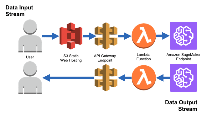
In this architecture, the client sends a request to API Gateway, which triggers a Lambda function. The Lambda function then invokes the SageMaker endpoint and returns the forecasts to the client. Several key benefits for this architecture:
Scalability: Automatically scales resources to meet the demand of inference requests. Ideal for applications with fluctuating or unpredictable traffic, ensuring that resources are efficiently utilized and not wasted during idle times.
Cost-Effective: Operates on a pay-per-use model. We only incur costs when the Lambda function is invoked and when the SageMaker endpoint processes requests. This is particularly advantageous for intermittent use cases, as there are no charges during idle periods.
Enhanced Security and Isolation: Each component (API Gateway, Lambda, SageMaker) provides built-in security features, contributing to a secure and isolated environment for processing and handling inference requests.
Model Serving & Serverless Endpoint
Serving Entry
Similar to processing and training jobs, we will use a Docker container to serve our model. First, we create a serve_entry.py (link) entrypoint in the src package. This script, leveraging FastAPI, forms the core of our serving logic. Below is an overview:
| Section | Description |
|---|---|
| Script Overview | The serve_entry.py script is set up for serving a machine learning model using FastAPI, a modern framework for building APIs. It’s designed to be deployed as a containerized application, primarily for use with Amazon SageMaker’s serverless inference endpoints. |
| Key Libraries Used | - FastAPI: For creating RESTful APIs. - uvicorn: An ASGI server for FastAPI. - joblib: For loading serialized models. - pandas: For data manipulation and analysis. - sktime: For time series forecasting functionalities. |
| Application Lifespan Management | Implements an asynccontextmanager for managing the startup and shutdown of the FastAPI application, which includes loading the model, transformer, and data, as well as cleanup tasks. |
| Forecasting Logic | Provides a forecast function for predicting future values based on the model, taking periods and prediction interval coverage as inputs. The function uses the loaded model and Fourier transformer to generate forecasts and returns a JSON string with predictions and prediction intervals. |
| FastAPI Application Setup | Configures a FastAPI application with endpoints (/ping and /invocations) to handle health checks and inference requests. The /ping endpoint responds to health check requests from SageMaker, while the /invocations endpoint processes inference requests with JSON payloads containing forecasting parameters. |
| Endpoint Details | - /ping: Returns a simple JSON response to indicate the application’s health status.- /invocations: Accepts POST requests with a JSON payload specifying the forecasting parameters and returns the forecast results in JSON format. |
| Error Handling and Validation | Includes error handling and input validation for the /invocations endpoint to ensure that incoming requests contain valid data. Errors are logged, and appropriate HTTP response codes are returned for different error types. |
| Application Execution | Uses uvicorn to run the FastAPI application, listening on port 8080. Configures logging and starts the application with the defined lifespan management and endpoints. |
| Model Loading and Usage | On startup, the script loads the trained model and Fourier transformer from disk. SageMaker copies these artifacts from the S3 path we provide onto the container at runtime. These components are used in the forecast function to generate predictions based on the input parameters. |
Docker
Add a serve.Dockerfile in the docker directory. This file, differing slightly from the preprocess.Dockerfile and train.Dockerfile, specifies serve_entry.py as the entrypoint and includes necessary libraries:
FROM python:3.10.12-slim-bullseye

WORKDIR /opt/ml/code/

# Only copy files not listed in the dockerfile specific .dockerignore file
COPY ./src/ ./

RUN pip install pandas[performance]==1.5.3 \
                sktime==0.24.0 \
                statsforecast==1.4.0 \
                hydra-core==1.3.2 \
                joblib==1.3.2 \
                fastapi==0.104.1 \
                uvicorn==0.24.0.post1

# Ensure python I/O is unbuffered so log messages are immediate
ENV PYTHONUNBUFFERED=True
# Disable the generation of bytecode '.pyc' files
ENV PYTHONDONTWRITEBYTECODE=True

ENTRYPOINT ["python3", "serve_entry.py"]
Add a serve.Dockerfile.ignore to the docker directory. While this is very similar to train.Dockerfile.ignore and preprocess.Dockerfile.ignore, it does not necessarily have to be, and so the separation of logic may still be useful in the future if we want to ignore different files for processing, training, and serving:
src/*
!src/config
!src/serve_entry.py
!src/custom_utils.py
Build and push the serving docker image to ECR and construct the serving image uri:
!cd {config['docker_dir_path']} && bash ./build_and_push.sh serve-latest serve {config['ecr_repository']}

# Construct serving image uri
images = !aws ecr list-images --repository-name {config['ecr_repository']}
images_str = '\n'.join(images)
images_str = json.loads(images_str)

for ecr_meta_data_dict in images_str['imageIds']:
    if ecr_meta_data_dict['imageTag'].startswith('serve'):
        serve_image_tag = ecr_meta_data_dict['imageTag']

serve_image_uri = f'{sagemaker_session.account_id()}.dkr.ecr.{sagemaker_session.boto_region_name}.amazonaws.com/{config["ecr_repository"]}:{serve_image_tag}'
Model
Next, we create a SageMaker model instance, and use it to deploy the best model found during hyperparameter optimization as a serverless endpoint. The key parameters are:
Serving docker image
S3 path of the best model artifacts, which is stored as a variable
best_model_s3_pathin the previous section
More details on the Model API here.
best_model = Model(
    image_uri=serve_image_uri,
    model_data=best_model_s3_path,
    role=role,
    name=config['serve_model_name'],
    code_location=config['code_location'],
    sagemaker_session=sagemaker_session
)
Serverless Endpoint Configuration & Deployment
Instantiate the ServerlessInferenceConfig class, which has two key parameters:
memory_size_in_mb(int): This parameter sets the memory size available to the serverless endpoint. We can choose from predefined sizes, ranging in 1 GB increments, such as 1024 MB, 2048 MB, and so on, up to 6144 MB.max_concurrency(int): This parameter defines the maximum number of concurrent invocations that the serverless endpoint can handle. It essentially determines how many requests the endpoint can process at the same time.
serverless_inference_config = ServerlessInferenceConfig(
    memory_size_in_mb=config['serve_memory_size_in_mb'],
    max_concurrency=config['serve_max_concurrency']
)
Explore more about serverless inference:
Serverless Inference with Amazon SageMaker
API for the
ServerlessInferenceConfigclass
Finally, deploy the model as a serverless endpoint:
best_model.deploy(
    initial_instance_count=config['serve_initial_instance_count'],
    instance_type=config['serve_instance_type'],
    endpoint_name=config['serve_endpoint_name'],
    serverless_inference_config=serverless_inference_config,
    volume_size=config['serve_volume_size'],
    wait=True # Wait until the deployment finishes
)----------!AWS Lambda
The serverless endpoint deployed in the previous section is a great way to get started with serverless inference. However, it remains non-trivial for a client to make inference requests to the endpoint hosting our trained model. In this section, we will create a Lambda function serving as a doorman to the serverless endpoint. The Lambda function will be responsible for invoking the serverless endpoint, effectively managing the communication between any inference requests and the serverless endpoint.
Lambda Function
The Lambda function is defined in the lambda_function.py (link) module. The table below provides an overview of the key components of the Lambda function:
| Section | Description |
|---|---|
| Function Overview | The lambda_handler function is the entry point for AWS Lambda execution. It processes the event data received when the function is invoked. |
| Event Object | The event is a JSON-formatted object provided by AWS Lambda. It contains data about the invocation, such as API Gateway request data, in the case of an API-triggered Lambda. |
| Context Parameter | The context parameter provides runtime information about the Lambda execution, such as execution deadline, function ARN, etc. |
| Key Libraries Used | boto3 (AWS SDK for Python) |
| Invocation Process | Extracts the payload from the event, invokes the SageMaker endpoint with the payload, and returns the response. |
| Error Handling | Implements error handling to manage potential issues during the invocation process. |
The lambda_function.py module is the source code for the lambda function, which we will deploy in the next step. For more details, see the official documentations on building Lambda functions with Python.
Lambda Manager Class
The LambdaManager (see ?LambdaManager for details) class from the lambda_manager.py (link) module contains methods to create, deploy, update, and delete lambda functions using boto3.
- To integrate AWS Lambda with our serverless model endpoint, we first establish an execution role, which we created in the Lambda Execution Role section. This role grants the necessary permissions for the Lambda function to interact with other AWS services, such as Amazon SageMaker:
lambda_manager = LambdaManager(
    lambda_client=lambda_boto3,
    iam_resource=iam_boto3
)

# Use the execution role we created for the lambda function
lambda_execution_role, exist = lambda_manager.create_iam_role_for_lambda(
    iam_role_name=config['lambda_execution_role_name']
)
2023-11-21 08:32:59,203 INFO src.lambda_manager: Found IAM role forecast-lambda-execution-role- Next, we prepare a deployment package, which includes the source code for the Lambda function. This package is created as a
bytesobject in memory for deployment:
deployment_package = lambda_manager.create_deployment_package(
    source_file=os.path.join(config['src_dir_path'], config['lambda_source_file']),
    destination_file=config['lambda_source_file']
)

type(deployment_package)bytes- With the deployment package ready, we proceed to create and deploy the Lambda function. This involves specifying various parameters like function name, description, runtime, and the IAM role:
lambda_function_arn = lambda_manager.create_function(
    function_name=config['lambda_function_name'],
    function_description=config['lambda_function_description'],
    time_out=config['lambda_time_out'],
    python_runtime=config['lambda_python_runtime'],
    iam_role=lambda_execution_role,
    handler_name=config['lambda_handler_name'],
    deployment_package=deployment_package,
    publish=config['lambda_publish'],
    # The configuration structures the env_vars as a list of dicts, but the SDK expects a single dict of key-value pairs
    env_vars={env_key: env_value for dict_obj in config['lambda_env_vars']
                                 for env_key, env_value in dict_obj.items()}
)
2023-11-21 08:33:08,853 INFO src.lambda_manager: Function forecast-lambda is active with ARN arn:aws:lambda:us-east-1:722696965592:function:forecast-lambdaBefore integrating our Lambda function with the REST API, we test the function with a sample payload to ensure that it is functioning as expected. The payload that the
serve_entry.pyexpects is a json object with abodykey, which is in and of itself a json object with two keys:periods: the number of periods to forecastsconf: the prediction interval coverage for the forecasts
response = lambda_manager.invoke_function(
    function_name=config['lambda_function_name'],
    payload={'body': json.dumps({'periods': '10', 'conf': '0.90'})},
    include_log=False
)

response_payload = json.loads(response['Payload'].read().decode('utf-8'))
predictions = json.loads(response_payload['body'])

pd.DataFrame.from_dict(predictions)
2023-11-21 08:33:38,048 INFO src.lambda_manager: Invoked function forecast-lambda| date | lower_pi_0.9 | predictions | upper_pi_0.9 | |
|---|---|---|---|---|
| 0 | 2023-11-10 | 8442.032846 | 8799.959536 | 9173.061660 |
| 1 | 2023-11-17 | 8407.632972 | 8764.101170 | 9135.682966 |
| 2 | 2023-11-24 | 8180.724608 | 8533.211927 | 8900.887059 |
| 3 | 2023-12-01 | 8377.697623 | 8746.039429 | 9130.576101 |
| 4 | 2023-12-08 | 8570.751497 | 8954.925552 | 9356.319766 |
| 5 | 2023-12-15 | 8623.091041 | 9016.872044 | 9428.635402 |
| 6 | 2023-12-22 | 8017.558637 | 8390.324085 | 8780.420754 |
| 7 | 2023-12-29 | 7801.960859 | 8171.054973 | 8557.610142 |
| 8 | 2024-01-05 | 7836.116017 | 8213.105585 | 8608.231835 |
| 9 | 2024-01-12 | 7993.866235 | 8384.753272 | 8794.754048 |
REST API
In this section, we explore the integration of AWS API Gateway with Lambda, a key component in handling requests to our serverless inference endpoint. AWS API Gateway serves as the front-end interface for our Lambda function. This setup is crucial as it enables us to expose our backend model endpoint to external applications.
Through this integration, clients can seamlessly make inference requests, allowing for efficient and scalable interaction with our model hosted on AWS. The API Gateway acts not just as a mere conduit but also offers additional features like request routing, security, usage plan, and monitoring, thereby enhancing the overall functionality and reliability of the serverless architecture.
With API’s, we can also control how clients call an API, using IAM permissions, a Lambda authorizer, or an Amazon Cognito user pool.
Usage Plans
One of the key benefits of using AWS API Gateway in conjunction with Lambda is the ability to specify usage plans. These plans are instrumental in managing how clients interact with our API.
Controlled Access: We utilize usage plans to dictate how our APIs are used, associating API keys with these plans to manage access frequency. This is especially beneficial for offering different access levels to various users.
Efficient Throttling and Quotas: Our usage plans include throttling rules to limit request numbers over set periods, along with quota limits. This approach ensures equitable resource use and maintains performance.
Customizability: We can tailor usage plans to meet the varying needs of our audience, balancing accessibility and resource management, whether for internal, partner, or commercial use.
In this project, we implement a simple usage plan with a single API key and a throttling rate of 10 requests per second. This plan is sufficient for our purposes, but we can easily expand it to include more API keys and additional throttling rules.
REST API Setup and Management
Using the RestApiManager class from the rest_api_manager.py (link) module, we streamline the creation and management of our REST API on AWS API Gateway. This class encapsulates various steps required to set up and manage an API, ensuring a seamless and efficient process.
We begin by instantiating the
RestApiManagerclass, specifying parameters like API name, base path, stage, and Lambda function name. These parameters define the basic structure of our API.Create REST API: Initializes a new API on AWS API Gateway, laying the foundation for external applications to interact with our lambda function. Learn more about REST APIs in API Gateway.
Get Root Resource ID: Retrieves the root resource ID of the API, which is crucial for constructing URL paths within our API. This will be needed to ultimately invoke the API for inference requests. Understand Resources and Methods in API Gateway
Create Resource: Adds a new endpoint under the root resource, defining specific URL paths and their handling within the API. Create Resources and Methods.
Create POST Method: Establishes a POST method for the new resource, including API key requirements and other configurations. We use a POST method since the client will be sending data to the Lambda function. Setting up POST Method in API Gateway.
Setup Lambda Integration: Integrates the API with our AWS Lambda function, enabling the POST method to trigger the Lambda function, which invokes the backend inference endpoint. Integrate API with AWS Lambda.
Deploy REST API: Makes the API publicly accessible through deployment, making it available to end users. Deploying Our API.
Grant Permission to Lambda: Authorizes API Gateway to invoke our specified Lambda function, ensuring secure interaction between these two services. Manage Lambda Permissions.
API Key and Usage Plan Setup: Creates API keys and usage plans for controlling access, quotas, and rate limits on the individual API key. API Keys and Usage Plans in API Gateway.
rest_api_manager = RestApiManager(
    api_name=config['api_gateway_api_name'],
    api_base_path=config['api_gateway_api_base_path'],
    api_stage=config['api_gateway_api_stage'], # Development stage
    lambda_function_name=config['lambda_function_name']
)

rest_api_manager.setup_rest_api(
    apiKeyRequired=config['api_gateway_api_key_required'],
    api_key_name=config['api_gateway_api_key_name'],
    enabled=config['api_gateway_enabled'],
    usage_plan_name=config['api_gateway_usage_plan_name']
)
2023-11-21 08:33:43,972 INFO src.rest_api_manager: Created REST API forecast-api with ID ho0bqqd0x1
2023-11-21 08:33:44,017 INFO src.rest_api_manager: Found root resource of the REST API with ID oxpzkbuc7c
2023-11-21 08:33:44,074 INFO src.rest_api_manager: Created resource forecast under root resource with ID 4ev4qp
2023-11-21 08:33:44,133 INFO src.rest_api_manager: Created POST method for resource 4ev4qp
2023-11-21 08:33:44,199 INFO src.rest_api_manager: Set up Lambda integration for POST method on resource 4ev4qp
2023-11-21 08:33:44,674 INFO src.rest_api_manager: Deployed REST API ho0bqqd0x1
2023-11-21 08:33:44,753 INFO src.rest_api_manager: Granted permission to let Amazon API Gateway invoke function arn:aws:lambda:us-east-1:722696965592:function:forecast-lambda from arn:aws:execute-api:us-east-1:722696965592:ho0bqqd0x1/*/POST/forecast
2023-11-21 08:33:44,807 INFO src.rest_api_manager: Created API key with ID vivx7v165i
2023-11-21 08:33:45,412 INFO src.rest_api_manager: Created usage plan with ID p75ul0
2023-11-21 08:33:45,781 INFO src.rest_api_manager: Added API key vivx7v165i to usage plan p75ul0
2023-11-21 08:33:45,782 INFO src.rest_api_manager: Finished setting up REST API- Invoke the REST API, if an
api_keyis required, then this method (i.e.,invoke_rest_api) automatically adds theapi_keyto the header of the request sent to API Gateway:
payload = {'periods': '5', 'conf': '0.80'}

predictions = rest_api_manager.invoke_rest_api(
    payload=payload
)

pd.DataFrame.from_dict(predictions)
2023-11-21 08:36:24,683 INFO src.rest_api_manager: Constructed REST API base URL: https://ho0bqqd0x1.execute-api.us-east-1.amazonaws.com/dev/forecast
2023-11-21 08:36:25,138 INFO src.rest_api_manager: Invoked REST API ho0bqqd0x1 with payload {'periods': '5', 'conf': '0.80'} and API key vivx7v165i| date | lower_pi_0.8 | predictions | upper_pi_0.8 | |
|---|---|---|---|---|
| 0 | 2023-11-10 | 8519.814962 | 8799.959536 | 9089.315693 |
| 1 | 2023-11-17 | 8485.098139 | 8764.101170 | 9052.278249 |
| 2 | 2023-11-24 | 8257.304785 | 8533.211927 | 8818.338150 |
| 3 | 2023-12-01 | 8457.695795 | 8746.039429 | 9044.213406 |
| 4 | 2023-12-08 | 8654.161291 | 8954.925552 | 9266.142490 |
That is it. We now have a fully functional REST API that can be used to generate forecasts.
Checkpoint VI
The final project directory should now resemble:
.
├── docker
│   ├── build_and_push.sh
│   ├── preprocess.Dockerfile
│   ├── preprocess.Dockerfile.dockerignore
│   ├── serve.Dockerfile
│   ├── serve.Dockerfile.dockerignore
│   ├── train.Dockerfile
│   └── train.Dockerfile.dockerignore
├── notebooks
│   ├── eda.ipynb
│   └── forecast.ipynb
├── poetry.lock
├── pyproject.toml
├── README.md
├── src
│   ├── config
│   │   └── main.yaml
│   ├── custom_utils.py
│   ├── lambda_function.py
│   ├── lambda_manager.py
│   ├── preprocess_entry.py
│   ├── rest_api_manager.py
│   ├── serve_entry.py
│   └── train_entry.py
└── tests
    └── __init__.py
Important: Clean-Up
To clean up the resources we created:
- Remove the preprocessing and training images:
for image_tag in [train_image_tag, preprocess_image_tag, serve_image_tag]:
    ecr_boto3.batch_delete_image(
        repositoryName=config['ecr_repository'],
        imageIds=[{'imageTag': image_tag}]
)- Delete model, serverless endpoint, and serverless endpoint configuration:
sm_boto3.delete_endpoint(EndpointName=config['serve_endpoint_name'])
sm_boto3.delete_endpoint_config(EndpointConfigName=config['serve_endpoint_name'])
sm_boto3.delete_model(ModelName=config['serve_model_name'])
{'ResponseMetadata': {'RequestId': '9e42a2af-c22d-4205-b467-9f4732f0f05b',
'HTTPStatusCode': 200,
'HTTPHeaders': {'x-amzn-requestid': '9e42a2af-c22d-4205-b467-9f4732f0f05b',
'content-type': 'application/x-amz-json-1.1',
'content-length': '0',
'date': 'Tue, 21 Nov 2023 08:36:55 GMT'},
'RetryAttempts': 0}}- Remove lambda function:
lambda_manager.delete_function(function_name=config['lambda_function_name'])2023-11-21 08:36:58,437 INFO src.lambda_manager: Deleted function forecast-lambda- Clean up resources related to REST API:
rest_api_manager.cleanup()2023-11-21 08:37:00,506 INFO src.rest_api_manager: Cleaning up resources created during the setup process
2023-11-21 08:37:00,507 INFO src.rest_api_manager: Rolling back created resources
2023-11-21 08:37:00,529 INFO src.rest_api_manager: Nothing to remove as the specified Lambda function does not exist
2023-11-21 08:37:00,811 INFO src.rest_api_manager: Deleted API key vivx7v165i from usage plan p75ul0
2023-11-21 08:37:00,870 INFO src.rest_api_manager: Deleted resource 4ev4qp
2023-11-21 08:37:01,122 INFO src.rest_api_manager: Deleted REST API ho0bqqd0x1
2023-11-21 08:37:01,466 INFO src.rest_api_manager: Deleted usage plan p75ul0
2023-11-21 08:37:01,684 INFO src.rest_api_manager: Deleted API key vivx7v165i- Close clients:
ecr_boto3.close()
sm_boto3.close()
apigateway_boto3.close()
lambda_boto3.close()
Putting it all together
After navigating through the intricacies of setting up IAM roles, configuring AWS resources, conducting exploratory data analysis, and training and deploying models using AWS Lambda and API Gateway, we have created a end-to-end machine learning pipeline.
For a comprehensive view of the complete process, all source files are available at this GitHub repository. This repository serves as a practical blueprint, illustrating how each component integrates into an end-to-end machine learning solution for time series forecasting using AWS SageMaker and associated services.
Resources
FastAPI and Serverless Deployment
- FastAPI Advanced Events: Detailed guidance on advanced usage of FastAPI, including event handling.
- R Serving with FastAPI - Example: A practical example of serving R models with FastAPI.
- SageMaker Serverless Inference Documentation: Python API.
- Amazon SageMaker Inference Code: Guidance on writing inference code for SageMaker models.
SageMaker and AWS Services
- SageMaker Python SDK: Python API for SageMaker.
- Boto3 API Gateway Documentation: Python API for API Gateway.
- Boto3 Lambda Documentation: Python API for Lambda.
- Invoking Serverless Endpoints: Instructions on how to invoke SageMaker serverless endpoints.
- Adapting Docker Containers for SageMaker: Learn how to adapt your Docker containers for SageMaker for both training and inference.
- Creating Docker Containers for SageMaker: Learn how to create Docker containers for SageMaker for both training and inference.
- AWS Lambda Python Code Examples: Various Python examples for AWS Lambda functions.
- Calling SageMaker Endpoints via API Gateway and Lambda: A blog post illustrating the integration of SageMaker, API Gateway, and Lambda.
- API Gateway and Lambda Integration: Example code for integrating API Gateway with Lambda.
IAM and Security
- IAM Policy Reference: A comprehensive reference for IAM policies for all AWS services.
- IAM Policy Grammar: Understand the grammar and structure of IAM policies.
- Lambda Access Control: Information on access control for Lambda functions.
Time Series Analysis and Forecasting
- Rob J Hyndman’s Blog: Insights and tutorials on time series analysis from a leading expert.
- Forecasting: Principles and Practice: A comprehensive online textbook on forecasting methods.
- Time Series Analysis: With Applications in R: A comprehensive, theoretically-rigorous textbook on time series analysis.
Python Time Series Libraries
- sktime: A Unified Interface for Machine Learning with Time Series: An open-source Python library for time series analysis.
- statsforecast: Fast Univariate Time Series Forecasting: A Python library for efficient forecasting of univariate time series.
- statsmodels: Time Series Analysis: Python statistical library that provides classes and functions for time series analysis.
- pmdarima: ARIMA estimators for Python: A Python library for auto-regressive integrated moving average models.